Data Mining and Data Discovery from Dog Breeds Data

14 minute read

Discovering New Data from Dog Breeds

I wanted to do this project wanting to explore some data mining techniques and visualizations on a dataset of dog breeds and their various features and characteristics. I started this project by importing some Python data processing libraries.

import pandas as pd
import numpy as np
import sklearn
from matplotlib import pyplot as plt
import seaborn as sns
from sklearn.feature_extraction.text import TfidfVectorizer
from sklearn.feature_extraction.text import CountVectorizer
from sklearn.preprocessing import OneHotEncoder
from sklearn.preprocessing import Normalizer
from sklearn.preprocessing import StandardScaler
from sklearn.decomposition import PCA
from sklearn.manifold import TSNE
from sklearn.cluster import KMeans

My first step is to look at the data in tabular form.

df = pd.read_csv('DogBreeds.csv')
df

	Name	Origin	Type	Unique Feature	Friendly Rating (1-10)	Life Span	Size	Grooming Needs	Exercise Requirements (hrs/day)	Good with Children	Intelligence Rating (1-10)	Shedding Level	Health Issues Risk	Average Weight (kg)	Training Difficulty (1-10)
0	Affenpinscher	Germany	Toy	Monkey-like face	7	14	Small	High	1.5	Yes	8	Moderate	Low	4.0	6
1	Afghan Hound	Afghanistan	Hound	Long silky coat	5	13	Large	Very High	2.0	No	4	High	Moderate	25.0	8
2	Airedale Terrier	England	Terrier	Largest of terriers	8	12	Medium	High	2.0	Yes	7	Moderate	Low	21.0	6
3	Akita	Japan	Working	Strong loyalty	6	11	Large	Moderate	2.0	With Training	7	High	High	45.0	9
4	Alaskan Malamute	Alaska USA	Working	Strong pulling ability	7	11	Large	High	3.0	Yes	6	Very High	Moderate	36.0	8
...	...	...	...	...	...	...	...	...	...	...	...	...	...	...	...
154	Wire Fox Terrier	England	Terrier	Energetic	7	14	Small	Moderate	2.0	Yes	7	Moderate	Moderate	8.0	7
155	Wirehaired Dachshund	Germany	Hound	Wiry coat	7	13	Small	Moderate	1.5	With Training	7	Moderate	High	8.0	7
156	Wirehaired Pointing Griffon	Netherlands	Sporting	Shaggy beard	7	13	Medium	High	2.0	Yes	7	Moderate	Moderate	20.0	6
157	Xoloitzcuintli	Mexico	Non-Sporting	Hairless variety	7	15	Small-Large	Low	2.0	With Training	8	Low	Moderate	25.0	6
158	Yorkshire Terrier	England	Toy	Long silky coat	8	13	Toy	High	1.0	Yes	7	Moderate	Moderate	2.5	6

159 rows × 15 columns

Data Exploration

From the table, I picked 5 features that I was most interested in to learn more about associations with dog breeds. The features I picked are:

Friendly rating
Training difficulty
Intelligence
Lifespan
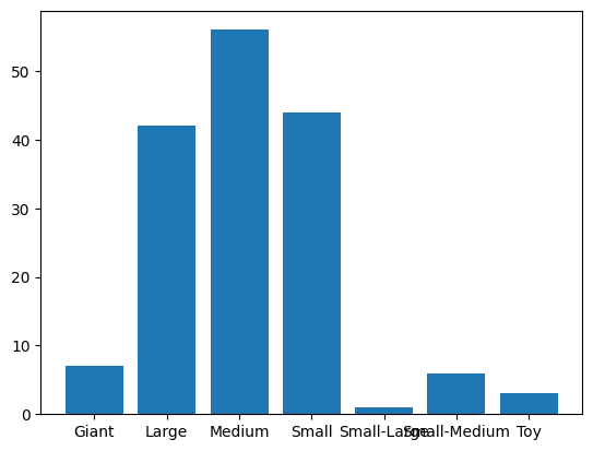
Size My plan is to try to generate some tables and graphs that can teach me something about these features. First I want to group the data by count of number of breeds for each size category.
```
grouped_df = df.groupby('Size')
grouped_df.get_group('Medium')
grouped_sizecounts = df.groupby('Size').count().select_dtypes('int')
grouped_sizecounts
```
The results of the grouping are as follows:

	Name	Origin	Type	Unique Feature	Friendly Rating (1-10)	Life Span	Grooming Needs	Exercise Requirements (hrs/day)	Good with Children	Intelligence Rating (1-10)	Shedding Level	Health Issues Risk	Average Weight (kg)	Training Difficulty (1-10)
Size
Giant	7	7	7	7	7	7	7	7	7	7	7	7	7	7
Large	42	42	42	42	42	42	42	42	42	42	42	42	42	42
Medium	56	56	56	56	56	56	56	56	56	56	56	56	56	56
Small	44	44	44	44	44	44	44	44	44	44	44	44	44	44
Small-Large	1	1	1	1	1	1	1	1	1	1	1	1	1	1
Small-Medium	6	6	6	6	6	6	6	6	6	6	6	6	6	6
Toy	3	3	3	3	3	3	3	3	3	3	3	3	3	3

Using the results of the size groupings, I chart a bar graph of the quantities of dog breeds for each size category.

sizes = ['Giant', 'Large', 'Medium', 'Small', 'Small-Large', 'Small-Medium', 'Toy']
counts = [7, 42, 56, 44, 1, 6, 3]
plt.bar(sizes, counts)
plt.show()

I used Seaborn as an advanced plotting and visualization library to display the count of dog breeds correlated between training difficulty and intelligence rating.

sns.countplot(x='Training Difficulty (1-10)', hue='Intelligence Rating (1-10)', data=df)

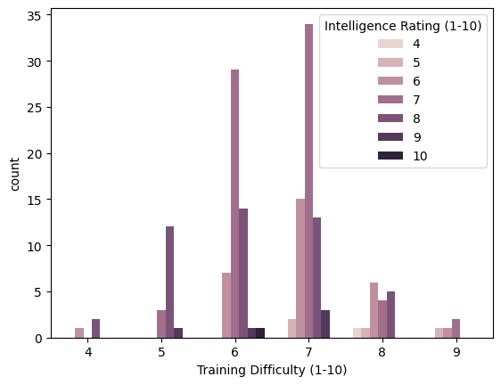
Some of the things we can learn from this bar plot and this data is that:

Most dogs have a 6 or 7 training difficulty level
The dogs with the highest training difficulty level have lower intelligence
Dogs with lower training difficulty level have higher intelligence

In addition to correlation between intelligence and training difficulty, I also want to see correlation between the intelligence and the friendliness

sns.countplot(x='Friendly Rating (1-10)', hue='Intelligence Rating (1-10)', data=df)

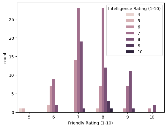
Some of the things I learned from this graph are:

According to count, almost all dogs are very friendly
Up to a point, higher intelligence can also correlate with a higher friendliness rating with the exception of the dogs with the highest friendliness rating which are moderately intelligent

Feature Extraction and Data Processing Approach

Feature Extraction
- We need to vectorize the data in order to produce vectors that can be projected into a visual space
  - For the text based data, we will use tfidf to vectorize text
  - for the ranking based data, we will encode all rankings based values into numerical classes and then normalize to a range between 0 and 1
- Then we will scale all features using the standard scaler
- After the data is vectorized then we can perform dimensionality reduction using pca and tsne

The first high level step is vectorize.
- As part of the process of vectorization, we need to vectorize the text using tfidf.
- The next step to vectorize the data is to encode rankings based values into numerical classes.
- The last step to vectorize the data is to normalize all ranking based values.
- This will complete the vectorization process.
The second high level step is scaling and dimensionality reduction.
- The first part of this process will be to scale all features using the standard scaler.
- The next part of this process will be to use pca (principle component analysis)
- The last step to perform the dimensionality reduction is to use tsne (T-distributed Stochastic Neighbor Embedding)
- This will complete the dimensionality reduction portion

I wrote this code to extract the textual data from the dataset and represented as the TF-IDF score which is the term frequency inverse document frequency score.

tfidf_converter = TfidfVectorizer(lowercase=True, max_features=4)
extracted_name = tfidf_converter.fit_transform(df['Name']).toarray()
extracted_origin = tfidf_converter.fit_transform(df['Origin']).toarray()
extracted_type = tfidf_converter.fit_transform(df['Type']).toarray()
extracted_feature = tfidf_converter.fit_transform(df['Unique Feature']).toarray()
df

Next we use the Pandas utility “get_dummies” to create an encoding of categorical data. This way categories of features that are ranked can be represented as numbers instead of text without needing to calculate the TF-IDF score.

df = pd.get_dummies(df, prefix=['Size'], columns=['Size'], drop_first=False, dtype=float)
df = pd.get_dummies(df, prefix=['Grooming Needs'], columns=['Grooming Needs'], drop_first=False, dtype=float)
df = pd.get_dummies(df, prefix=['Good with Children'], columns=['Good with Children'], drop_first=False, dtype=float)
df = pd.get_dummies(df, prefix=['Health Issues Risk'], columns=['Health Issues Risk'], drop_first=False, dtype=float)
df = pd.get_dummies(df, prefix=['Shedding Level'], columns=['Shedding Level'], drop_first=False, dtype=float)
df = df.drop('Name', axis=1)
df = df.drop('Origin', axis=1)
df = df.drop('Type', axis=1)
df = df.drop('Unique Feature', axis=1)
df

The numerically encoded data appears like this:

	Friendly Rating (1-10)	Life Span	Exercise Requirements (hrs/day)	Intelligence Rating (1-10)	Average Weight (kg)	Training Difficulty (1-10)	Size_Giant	Size_Large	Size_Medium	Size_Small	...	Good with Children_No	Good with Children_With Training	Good with Children_Yes	Health Issues Risk_High	Health Issues Risk_Low	Health Issues Risk_Moderate	Shedding Level_High	Shedding Level_Low	Shedding Level_Moderate	Shedding Level_Very High
0	7	14	1.5	8	4.0	6	0.0	0.0	0.0	1.0	...	0.0	0.0	1.0	0.0	1.0	0.0	0.0	0.0	1.0	0.0
1	5	13	2.0	4	25.0	8	0.0	1.0	0.0	0.0	...	1.0	0.0	0.0	0.0	0.0	1.0	1.0	0.0	0.0	0.0
2	8	12	2.0	7	21.0	6	0.0	0.0	1.0	0.0	...	0.0	0.0	1.0	0.0	1.0	0.0	0.0	0.0	1.0	0.0
3	6	11	2.0	7	45.0	9	0.0	1.0	0.0	0.0	...	0.0	1.0	0.0	1.0	0.0	0.0	1.0	0.0	0.0	0.0
4	7	11	3.0	6	36.0	8	0.0	1.0	0.0	0.0	...	0.0	0.0	1.0	0.0	0.0	1.0	0.0	0.0	0.0	1.0
...	...	...	...	...	...	...	...	...	...	...	...	...	...	...	...	...	...	...	...	...	...
154	7	14	2.0	7	8.0	7	0.0	0.0	0.0	1.0	...	0.0	0.0	1.0	0.0	0.0	1.0	0.0	0.0	1.0	0.0
155	7	13	1.5	7	8.0	7	0.0	0.0	0.0	1.0	...	0.0	1.0	0.0	1.0	0.0	0.0	0.0	0.0	1.0	0.0
156	7	13	2.0	7	20.0	6	0.0	0.0	1.0	0.0	...	0.0	0.0	1.0	0.0	0.0	1.0	0.0	0.0	1.0	0.0
157	7	15	2.0	8	25.0	6	0.0	0.0	0.0	0.0	...	0.0	1.0	0.0	0.0	0.0	1.0	0.0	1.0	0.0	0.0
158	8	13	1.0	7	2.5	6	0.0	0.0	0.0	0.0	...	0.0	0.0	1.0	0.0	0.0	1.0	0.0	0.0	1.0	0.0

159 rows × 27 columns

Now, with the textual data converted to TF-IDF vectors, and the categorical data encoded, I want each sample to be represented as a vector of all features combined from this data.

num_rows = df.shape[0]
rows = []
for i in range(num_rows):
    row = df.iloc[i].to_list()
    for j in range(len(extracted_name[i])):
        row.append(extracted_name[i][j])
        row.append(extracted_origin[i][j])
        row.append(extracted_type[i][j])
        row.append(extracted_feature[i][j])
    row = np.array(row)
    row = row.astype(np.float64)
    rows.append(row)
for row in rows:
    print(row)

After creating the feature vectors, I normalize them with the SKLearn library for normalization.

normalizer = Normalizer().fit(rows)
rows = normalizer.transform(rows)
for row in rows:
    print(row)

Lastly, to standardize the feature vectors, I use the standard scaler library.

scaler = StandardScaler().fit(rows)
rows = scaler.transform(rows)
for row in rows:
    print(row)

Now, to perform feature reduction, I use the principle component analysis technique, which should reduce the vector length for each sample.

pca = PCA(n_components=16).fit(rows)
rows = pca.transform(rows)
for row in rows:
    print(row)

Now that I have a standard feature representation for all samples, I want to map the feature space in 2 dimensions in a graph. I use the TSNE technique to plot each sample in 2 dimensions and visualize the space.

tsne = TSNE(n_components=2, perplexity=10, early_exaggeration=20, metric='cosine', random_state=None)
features = tsne.fit_transform(rows)
plt.figure(figsize=(10, 10))
plt.xlim(features[:, 0].min(), features[:, 0].max())
plt.ylim(features[:, 1].min(), features[:, 1].max())
for f in features:
    plt.plot(f[0], f[1], 'o')
plt.show(block=True)

Now that I have the samples plotted in 2 dimensions, I use the K Means algorithm to select centroids for each 7 clusters of samples based on how the plotted points appeared. It seemed like there were around 7 clusters from this graph.

k_means = KMeans(n_clusters=7, init='k-means++', n_init='auto', max_iter=300)
k_means_fit = k_means.fit(features)
plt.figure(figsize=(10, 10))
plt.xlim(features[:, 0].min(), features[:, 0].max())
plt.ylim(features[:, 1].min(), features[:, 1].max())
for f in features:
    plt.plot(f[0], f[1], 'o')
centroids = k_means_fit.cluster_centers_
for c in centroids:
    plt.plot(c[0], c[1], '+', color='black')
plt.show(block=True)

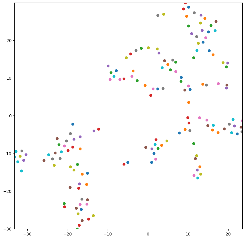
After the previous code segment, the K Means algorithm with K++ initialization chose these centroid positions to denote cluster centers. Using the centroids, I color code the samples based on distance to each centroid (unsupervised classification).

predicted = k_means_fit.predict(features)
plt.figure(figsize=(10, 10))
plt.xlim(features[:, 0].min(), features[:, 0].max())
plt.ylim(features[:, 1].min(), features[:, 1].max())
for i, f in enumerate(features):
    if predicted[i] == 0:
        plt.plot(f[0], f[1], 'o', color='red')
    if predicted[i] == 1:
        plt.plot(f[0], f[1], 'o', color='orange')
    if predicted[i] == 2:
        plt.plot(f[0], f[1], 'o', color='yellow')
    if predicted[i] == 3:
        plt.plot(f[0], f[1], 'o', color='green')
    if predicted[i] == 4:
        plt.plot(f[0], f[1], 'o', color='blue')
    if predicted[i] == 5:
        plt.plot(f[0], f[1], 'o', color='purple')
    if predicted[i] == 6:
        plt.plot(f[0], f[1], 'o', color='magenta')

centroids = k_means_fit.cluster_centers_
for c in centroids:
    plt.plot(c[0], c[1], '+', color='black')
plt.show(block=True)

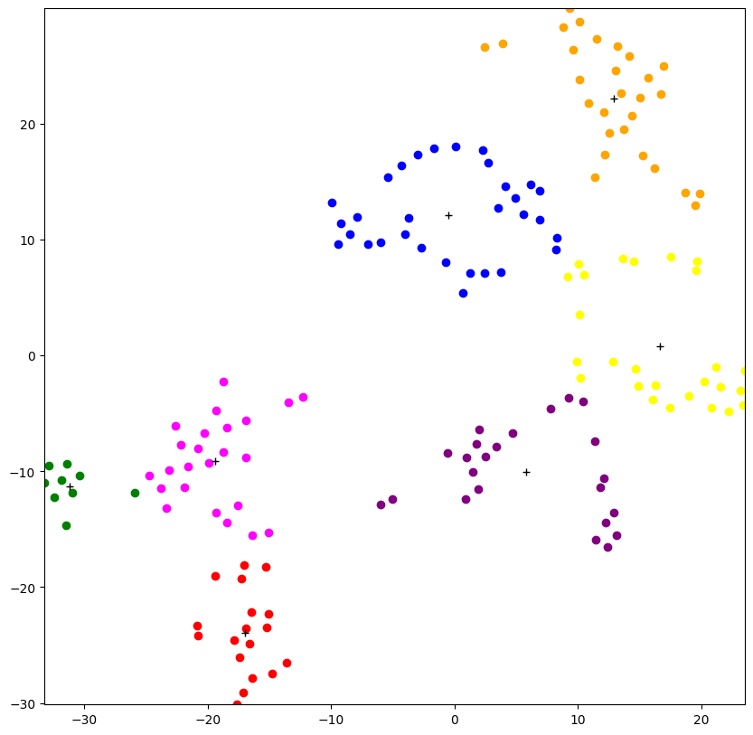
Now that the clusters have been organized and plotted on the graph, I can try to identify or interpret meaning from the assignment of each sample to a cluster. Since there are 7 clusters, I can try to select features that can be split into 7 different classes to predict meaning for the clusters. Features that are split in 7 different classes are size and intelligence. I can aggregate the ratio of similar predictions in each cluster for each class for size and intelligence to see how strongly our clusters are associated with those features.

index_0 = np.where(predicted == 0)
index_1 = np.where(predicted == 1)
index_2 = np.where(predicted == 2)
index_3 = np.where(predicted == 3)
index_4 = np.where(predicted == 4)
index_5 = np.where(predicted == 5)
index_6 = np.where(predicted == 6)

cluster_0_rows = df_new.iloc[index_0[0].tolist()]
cluster_1_rows = df_new.iloc[index_1[0].tolist()]
cluster_2_rows = df_new.iloc[index_2[0].tolist()]
cluster_3_rows = df_new.iloc[index_3[0].tolist()]
cluster_4_rows = df_new.iloc[index_4[0].tolist()]
cluster_5_rows = df_new.iloc[index_5[0].tolist()]
cluster_6_rows = df_new.iloc[index_6[0].tolist()]

cluster_0_freq_size = cluster_0_rows.Size.mode()
cluster_0_freq_int = cluster_0_rows["Intelligence Rating (1-10)"].mode()
cluster_1_freq_size = cluster_1_rows.Size.mode()
cluster_1_freq_int = cluster_1_rows["Intelligence Rating (1-10)"].mode()
cluster_2_freq_size = cluster_2_rows.Size.mode()
cluster_2_freq_int = cluster_2_rows["Intelligence Rating (1-10)"].mode()
cluster_3_freq_size = cluster_3_rows.Size.mode()
cluster_3_freq_int = cluster_3_rows["Intelligence Rating (1-10)"].mode()
cluster_4_freq_size = cluster_4_rows.Size.mode()
cluster_4_freq_int = cluster_4_rows["Intelligence Rating (1-10)"].mode()
cluster_5_freq_size = cluster_5_rows.Size.mode()
cluster_5_freq_int = cluster_5_rows["Intelligence Rating (1-10)"].mode()
cluster_6_freq_size = cluster_6_rows.Size.mode()
cluster_6_freq_int = cluster_6_rows["Intelligence Rating (1-10)"].mode()

cluster_0_size_matches = cluster_0_rows.loc[cluster_0_rows['Size'] == cluster_0_freq_size.iloc[0]]
cluster_1_size_matches = cluster_1_rows.loc[cluster_1_rows['Size'] == cluster_1_freq_size.iloc[0]]
cluster_2_size_matches = cluster_2_rows.loc[cluster_2_rows['Size'] == cluster_2_freq_size.iloc[0]]
cluster_3_size_matches = cluster_3_rows.loc[cluster_3_rows['Size'] == cluster_3_freq_size.iloc[0]]
cluster_4_size_matches = cluster_4_rows.loc[cluster_4_rows['Size'] == cluster_4_freq_size.iloc[0]]
cluster_5_size_matches = cluster_5_rows.loc[cluster_5_rows['Size'] == cluster_5_freq_size.iloc[0]]
cluster_6_size_matches = cluster_6_rows.loc[cluster_6_rows['Size'] == cluster_6_freq_size.iloc[0]]

cluster_0_int_matches = cluster_0_rows.loc[cluster_0_rows["Intelligence Rating (1-10)"] == cluster_0_freq_int.iloc[0]]
cluster_1_int_matches = cluster_1_rows.loc[cluster_1_rows["Intelligence Rating (1-10)"] == cluster_1_freq_int.iloc[0]]
cluster_2_int_matches = cluster_2_rows.loc[cluster_2_rows["Intelligence Rating (1-10)"] == cluster_2_freq_int.iloc[0]]
cluster_3_int_matches = cluster_3_rows.loc[cluster_3_rows["Intelligence Rating (1-10)"] == cluster_3_freq_int.iloc[0]]
cluster_4_int_matches = cluster_4_rows.loc[cluster_4_rows["Intelligence Rating (1-10)"] == cluster_4_freq_int.iloc[0]]
cluster_5_int_matches = cluster_5_rows.loc[cluster_5_rows["Intelligence Rating (1-10)"] == cluster_5_freq_int.iloc[0]]
cluster_6_int_matches = cluster_6_rows.loc[cluster_6_rows["Intelligence Rating (1-10)"] == cluster_6_freq_int.iloc[0]]

cluster_0_total_size = len(index_0[0])
cluster_0_match_size_len = len(cluster_0_size_matches.index)
cluster_0_size_accuracy = cluster_0_match_size_len / cluster_0_total_size
print(f'The accuracy score of cluster 0 size feature: {cluster_0_size_accuracy}')
cluster_1_total_size = len(index_1[0])
cluster_1_match_size_len = len(cluster_1_size_matches.index)
cluster_1_size_accuracy = cluster_1_match_size_len / cluster_1_total_size
print(f'The accuracy score of cluster 1 size feature: {cluster_1_size_accuracy}')
cluster_2_total_size = len(index_2[0])
cluster_2_match_size_len = len(cluster_2_size_matches.index)
cluster_2_size_accuracy = cluster_2_match_size_len / cluster_2_total_size
print(f'The accuracy score of cluster 2 size feature: {cluster_2_size_accuracy}')
cluster_3_total_size = len(index_3[0])
cluster_3_match_size_len = len(cluster_3_size_matches.index)
cluster_3_size_accuracy = cluster_3_match_size_len / cluster_3_total_size
print(f'The accuracy score of cluster 3 size feature: {cluster_3_size_accuracy}')
cluster_4_total_size = len(index_4[0])
cluster_4_match_size_len = len(cluster_4_size_matches.index)
cluster_4_size_accuracy = cluster_4_match_size_len / cluster_4_total_size
print(f'The accuracy score of cluster 4 size feature: {cluster_4_size_accuracy}')
cluster_5_total_size = len(index_5[0])
cluster_5_match_size_len = len(cluster_5_size_matches.index)
cluster_5_size_accuracy = cluster_5_match_size_len / cluster_5_total_size
print(f'The accuracy score of cluster 5 size feature: {cluster_5_size_accuracy}')
cluster_6_total_size = len(index_6[0])
cluster_6_match_size_len = len(cluster_6_size_matches.index)
cluster_6_size_accuracy = cluster_6_match_size_len / cluster_6_total_size
print(f'The accuracy score of cluster 6 size feature: {cluster_6_size_accuracy}')

All of the previous code is used to determine the number of matching samples that fall into a potential class that the clusters may match. These features are either the size or intelligence of the dog. The first output is a measure of how relevant the clustering is for the size feature. The results are as follows.

The accuracy score of cluster 0 size feature: 1.0
The accuracy score of cluster 1 size feature: 0.6071428571428571
The accuracy score of cluster 2 size feature: 0.6538461538461539
The accuracy score of cluster 3 size feature: 0.7777777777777778
The accuracy score of cluster 4 size feature: 0.5806451612903226
The accuracy score of cluster 5 size feature: 0.9130434782608695
The accuracy score of cluster 6 size feature: 0.9166666666666666

I used another similar code segment to determine the number of matching samples that fit the intelligence feature.

cluster_0_match_int_len = len(cluster_0_int_matches.index)
cluster_0_int_accuracy = cluster_0_match_int_len / cluster_0_total_size
print(f'The accuracy score of cluster 0 int feature: {cluster_0_int_accuracy}')
cluster_1_match_int_len = len(cluster_1_int_matches.index)
cluster_1_int_accuracy = cluster_1_match_int_len / cluster_1_total_size
print(f'The accuracy score of cluster 1 int feature: {cluster_1_int_accuracy}')
cluster_2_match_int_len = len(cluster_2_int_matches.index)
cluster_2_int_accuracy = cluster_2_match_int_len / cluster_2_total_size
print(f'The accuracy score of cluster 2 int feature: {cluster_2_int_accuracy}')
cluster_3_match_int_len = len(cluster_3_int_matches.index)
cluster_3_int_accuracy = cluster_3_match_int_len / cluster_3_total_size
print(f'The accuracy score of cluster 3 int feature: {cluster_3_int_accuracy}')
cluster_4_match_int_len = len(cluster_4_int_matches.index)
cluster_4_int_accuracy = cluster_4_match_int_len / cluster_4_total_size
print(f'The accuracy score of cluster 4 int feature: {cluster_4_int_accuracy}')
cluster_5_match_int_len = len(cluster_5_int_matches.index)
cluster_5_int_accuracy = cluster_5_match_int_len / cluster_5_total_size
print(f'The accuracy score of cluster 5 int feature: {cluster_5_int_accuracy}')
cluster_6_match_int_len = len(cluster_6_int_matches.index)
cluster_6_int_accuracy = cluster_6_match_int_len / cluster_6_total_size
print(f'The accuracy score of cluster 6 int feature: {cluster_6_int_accuracy}')

The relevance of the inteligence feature is measured below:

The accuracy score of cluster 0 int feature: 0.5
The accuracy score of cluster 1 int feature: 0.7857142857142857
The accuracy score of cluster 2 int feature: 0.5769230769230769
The accuracy score of cluster 3 int feature: 0.5555555555555556
The accuracy score of cluster 4 int feature: 0.5806451612903226
The accuracy score of cluster 5 int feature: 0.391304347826087
The accuracy score of cluster 6 int feature: 0.375

After comparing the relevance score of the size feature compared to the intelligence feature, by which each are measured as the ratio of samples that have matching classifications for each feature, I determined that the size feature is the more relevant feature that corresponds to the clustering and the visualization produced. Now with this in mind for my final analysis, I observe the actual category of size that was most frequent for each cluster.

print(f'The most common size for cluster 0 (red) is: {cluster_0_freq_size}')
print(f'The most common size for cluster 1 (orange) is: {cluster_1_freq_size}')
print(f'The most common size for cluster 2 (yellow) is: {cluster_2_freq_size}')
print(f'The most common size for cluster 3 (green) is: {cluster_3_freq_size}')
print(f'The most common size for cluster 4 (blue) is: {cluster_4_freq_size}')
print(f'The most common size for cluster 5 (purple) is: {cluster_5_freq_size}')
print(f'The most common size for cluster 6 (magenta) is: {cluster_6_freq_size}')

The most common size for cluster 0 (red) is: 0    Large
Name: Size, dtype: object
The most common size for cluster 1 (orange) is: 0    Small
Name: Size, dtype: object
The most common size for cluster 2 (yellow) is: 0    Medium
Name: Size, dtype: object
The most common size for cluster 3 (green) is: 0    Giant
Name: Size, dtype: object
The most common size for cluster 4 (blue) is: 0    Small
Name: Size, dtype: object
The most common size for cluster 5 (purple) is: 0    Medium
Name: Size, dtype: object
The most common size for cluster 6 (magenta) is: 0    Large
Name: Size, dtype: object

Results and Analysis

I found that the data of the dog breeds can be categorized into 7 clusters
The 7 clusters have a strong correlation with the size of the dog breeds
There are a range of sizes that are similar to each other (large and giant)
Versus some sizes very dissimilar to the large and giant dogs (small and medium)
The orange and blue clusters which are most frequently represented by small dogs are close together
The red, green and magenta clusters represent large dogs
The yellow and purple clusters represent medium dogs
The green cluster is located closest to the edge within all of the large dog clusters which shows how it represents the giant dogs

An-Jie Yu

Discovering New Data from Dog Breeds

Data Exploration

Feature Extraction and Data Processing Approach

Results and Analysis