
Drug Activity Classification and Prediction
Drug Activity Classification and Prediction on Numeric Sequential Data
This is a secondary intro to data mining project that explores more classification techniques and feature extraction and vectorization techniques on numeric data. First for this project, I import all the python libraries used.
import pandas as pd
import io
import numpy as np
import matplotlib.pyplot as plt
from math import isnan
from sklearn.tree import DecisionTreeClassifier
from sklearn.model_selection import train_test_split
from sklearn.metrics import accuracy_score, classification_report
from imblearn.under_sampling import RandomUnderSampler
from sklearn.decomposition import PCA
from sklearn.preprocessing import StandardScaler
After the python libraries are imported, I import the data from .txt sources and save them in a pandas dataframe.
file = io.open('train_data.txt', mode='r', encoding='utf-8')
text = file.read()
text = text.split('\n')
data = [line for line in text]

train_data_frame = pd.DataFrame(data, columns=['label'], dtype=pd.StringDtype())
train_data_frame[['label', 'activity']] = train_data_frame['label'].str.split('\t', n=1, expand=True)
samples = [tuple(np.fromstring(x, dtype=int, sep=' ')) for x in train_data_frame['activity']]
train_data_frame['activity'] = samples
train_data_frame
| label | activity | |
|---|---|---|
| 0 | 0 | (96, 183, 367, 379, 387, 1041, 1117, 1176, 132... |
| 1 | 0 | (31, 37, 137, 301, 394, 418, 514, 581, 671, 72... |
| 2 | 0 | (169, 394, 435, 603, 866, 1418, 1626, 1744, 17... |
| 3 | 0 | (72, 181, 231, 275, 310, 355, 369, 379, 400, 5... |
| 4 | 0 | (37, 379, 453, 503, 547, 611, 684, 716, 794, 8... |
| ... | ... | ... |
| 795 | 1 | (39, 120, 345, 400, 412, 558, 729, 1153, 1176,... |
| 796 | 0 | (43, 51, 280, 356, 378, 543, 557, 640, 666, 70... |
| 797 | 0 | (63, 232, 360, 405, 433, 447, 474, 751, 1069, ... |
| 798 | 0 | (83, 159, 290, 462, 505, 509, 531, 547, 737, 9... |
| 799 | 0 | (91, 432, 433, 509, 559, 578, 1082, 1153, 1220... |
800 rows × 2 columns
Now we can observe what are data is and explain what it represents. Each data point is a hypothetical amino chain of molecules represented as numbers, and the labels represent if the chain indicates the presence of a drug that the user is on. If the label is 0, there is no drug activity. If the label is 1, the amino chain indicates the presence of the drug. This project is about exploring feature extraction techniques that create a reliable classifier for this problem.
From this data, I can tell that there is an uneven distribution of negative to positive samples. There are far more amino chains that do not indicate drug activity. Therefore, another challenging aspect of this problem is the imbalanced data.
The first feature I want to observe is the length of each chain.
lengths = [len(x) for x in train_data_frame['activity']]
train_data_frame['length'] = lengths
train_data_frame
| label | activity | length | |
|---|---|---|---|
| 0 | 0 | (96, 183, 367, 379, 387, 1041, 1117, 1176, 132... | 732 |
| 1 | 0 | (31, 37, 137, 301, 394, 418, 514, 581, 671, 72... | 865 |
| 2 | 0 | (169, 394, 435, 603, 866, 1418, 1626, 1744, 17... | 760 |
| 3 | 0 | (72, 181, 231, 275, 310, 355, 369, 379, 400, 5... | 1299 |
| 4 | 0 | (37, 379, 453, 503, 547, 611, 684, 716, 794, 8... | 925 |
| ... | ... | ... | ... |
| 795 | 1 | (39, 120, 345, 400, 412, 558, 729, 1153, 1176,... | 770 |
| 796 | 0 | (43, 51, 280, 356, 378, 543, 557, 640, 666, 70... | 1835 |
| 797 | 0 | (63, 232, 360, 405, 433, 447, 474, 751, 1069, ... | 710 |
| 798 | 0 | (83, 159, 290, 462, 505, 509, 531, 547, 737, 9... | 864 |
| 799 | 0 | (91, 432, 433, 509, 559, 578, 1082, 1153, 1220... | 864 |
800 rows × 3 columns
The first attempts at feature extraction have to do with learning about the chain as a whole, by calculating values such as sum, average, minimum, and maximum.
sums = [sum(x) for x in train_data_frame['activity']]
train_data_frame['sum'] = sums
train_data_frame
| label | activity | length | sum | |
|---|---|---|---|---|
| 0 | 0 | (96, 183, 367, 379, 387, 1041, 1117, 1176, 132... | 732 | 37144141 |
| 1 | 0 | (31, 37, 137, 301, 394, 418, 514, 581, 671, 72... | 865 | 43919301 |
| 2 | 0 | (169, 394, 435, 603, 866, 1418, 1626, 1744, 17... | 760 | 38952818 |
| 3 | 0 | (72, 181, 231, 275, 310, 355, 369, 379, 400, 5... | 1299 | 62965542 |
| 4 | 0 | (37, 379, 453, 503, 547, 611, 684, 716, 794, 8... | 925 | 44947027 |
| ... | ... | ... | ... | ... |
| 795 | 1 | (39, 120, 345, 400, 412, 558, 729, 1153, 1176,... | 770 | 39040873 |
| 796 | 0 | (43, 51, 280, 356, 378, 543, 557, 640, 666, 70... | 1835 | 91516378 |
| 797 | 0 | (63, 232, 360, 405, 433, 447, 474, 751, 1069, ... | 710 | 35450063 |
| 798 | 0 | (83, 159, 290, 462, 505, 509, 531, 547, 737, 9... | 864 | 43486402 |
| 799 | 0 | (91, 432, 433, 509, 559, 578, 1082, 1153, 1220... | 864 | 44785955 |
800 rows × 4 columns
mins = [min(x) for x in train_data_frame['activity']]
train_data_frame['min'] = mins
maxs = [max(x) for x in train_data_frame['activity']]
train_data_frame['max'] = maxs
averages = [np.average(x) for x in train_data_frame['activity']]
train_data_frame['average'] = averages
train_data_frame
| label | activity | length | sum | min | max | average | |
|---|---|---|---|---|---|---|---|
| 0 | 0 | (96, 183, 367, 379, 387, 1041, 1117, 1176, 132... | 732 | 37144141 | 96 | 99875 | 50743.362022 |
| 1 | 0 | (31, 37, 137, 301, 394, 418, 514, 581, 671, 72... | 865 | 43919301 | 31 | 99932 | 50773.758382 |
| 2 | 0 | (169, 394, 435, 603, 866, 1418, 1626, 1744, 17... | 760 | 38952818 | 169 | 99875 | 51253.707895 |
| 3 | 0 | (72, 181, 231, 275, 310, 355, 369, 379, 400, 5... | 1299 | 62965542 | 72 | 99956 | 48472.318707 |
| 4 | 0 | (37, 379, 453, 503, 547, 611, 684, 716, 794, 8... | 925 | 44947027 | 37 | 99990 | 48591.380541 |
| ... | ... | ... | ... | ... | ... | ... | ... |
| 795 | 1 | (39, 120, 345, 400, 412, 558, 729, 1153, 1176,... | 770 | 39040873 | 39 | 99907 | 50702.432468 |
| 796 | 0 | (43, 51, 280, 356, 378, 543, 557, 640, 666, 70... | 1835 | 91516378 | 43 | 99991 | 49872.685559 |
| 797 | 0 | (63, 232, 360, 405, 433, 447, 474, 751, 1069, ... | 710 | 35450063 | 63 | 99955 | 49929.666197 |
| 798 | 0 | (83, 159, 290, 462, 505, 509, 531, 547, 737, 9... | 864 | 43486402 | 83 | 99829 | 50331.483796 |
| 799 | 0 | (91, 432, 433, 509, 559, 578, 1082, 1153, 1220... | 864 | 44785955 | 91 | 99945 | 51835.596065 |
800 rows × 7 columns
Now that some features have been calculated from the amino chain, next I try to visualize relationships between the positive and negative samples according to their features.
inactive_filter = train_data_frame['label'] == '0'
active_filter = train_data_frame['label'] == '1'
inactive_x = [x for x in train_data_frame['min'].where(inactive_filter)]
active_x = [x for x in train_data_frame['min'].where(active_filter)]
inactive_y = [y for y in train_data_frame['length'].where(inactive_filter)]
active_y = [y for y in train_data_frame['length'].where(active_filter)]
plt.plot(inactive_x, inactive_y, 'o')
plt.plot(active_x, active_y, 'o')
plt.xlabel('Min')
plt.ylabel('Length')
plt.show()
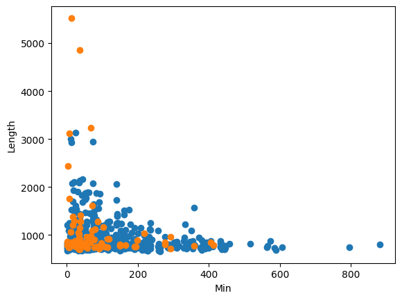
This plot does not reveal anything insightful about the features other than displaying our data imbalance.
Instead, I take a different approach to try and learn about specific numbers in the sequence. First I try to collect the most frequent numbers in active versus inactive samples.
active_samples = [x for x in train_data_frame['activity'].where(active_filter)]
inactive_samples = [x for x in train_data_frame['activity'].where(inactive_filter)]
def term_frequencies(rows):
    dic = {}
    for row in rows:
        try:
            isnan(row)
        except:
            for num in row:
                if num in dic:
                    dic[num] = dic[num] + 1
                else:
                    dic[num] = 1
    return dic
active_frequencies = term_frequencies(active_samples)
inactive_frequencies = term_frequencies(inactive_samples)
sorted_active_freqs = sorted(active_frequencies, key=active_frequencies.get, reverse=True)
sorted_inactive_freqs = sorted(inactive_frequencies, key=inactive_frequencies.get, reverse=True)
most_common_active_terms = set()
most_common_inactive_terms = set()
print('Most frequent numbers in active samples')
for freq in sorted_active_freqs:
    if (active_frequencies[freq] > 25):
        print(freq, active_frequencies[freq])
        most_common_active_terms.add(freq)
print('Most frequent numbers in inactive samples')
for freq in sorted_inactive_freqs:
    if (inactive_frequencies[freq] > 25):
        print(freq, inactive_frequencies[freq])
        most_common_inactive_terms.add(freq)
Most frequent numbers in active samples
412 46
81610 39
2526 38
25762 38
80131 35
92539 35
75364 33
44380 30
45474 29
50184 29
33876 28
28052 28
50522 26
Most frequent numbers in inactive samples
36005 187
9015 157
1176 149
14216 147
75393 142
32199 141
31192 134
54021 130
9197 128
55283 127
...
46635 26
83031 26
23619 26
91547 26
Using this new approach, I analyzed the frequent terms in amino chains for negative and positive samples. The results appear promising but in order to double check, I make sure that there is no overlap between terms in the negative versus positive samples.
shared_terms = most_common_active_terms.intersection(most_common_inactive_terms)
print(shared_terms)
set()
This is a very promising result because it means that there is no overlap between these frequent terms. My next approach is to use flags that indicate whether one of these most active terms is present, and to use that for my features.
train_data_frame['inactive_flags'] = train_data_frame['activity'].apply(lambda x : [1 if y in most_common_inactive_terms else 0 for y in x])
train_data_frame['active_flags'] = train_data_frame['activity'].apply(lambda x : [1 if y in most_common_active_terms else 0 for y in x])
train_data_frame
| label | activity | length | sum | min | max | average | inactive_flags | active_flags | |
|---|---|---|---|---|---|---|---|---|---|
| 0 | 0 | (96, 183, 367, 379, 387, 1041, 1117, 1176, 132... | 732 | 37144141 | 96 | 99875 | 50743.362022 | [1, 0, 0, 1, 0, 0, 0, 1, 0, 0, 0, 0, 0, 0, 0, ... | [0, 0, 0, 0, 0, 0, 0, 0, 0, 0, 0, 0, 0, 0, 0, ... |
| 1 | 0 | (31, 37, 137, 301, 394, 418, 514, 581, 671, 72... | 865 | 43919301 | 31 | 99932 | 50773.758382 | [0, 1, 0, 0, 0, 0, 0, 0, 1, 0, 0, 0, 0, 1, 0, ... | [0, 0, 0, 0, 0, 0, 0, 0, 0, 0, 0, 0, 0, 0, 0, ... |
| 2 | 0 | (169, 394, 435, 603, 866, 1418, 1626, 1744, 17... | 760 | 38952818 | 169 | 99875 | 51253.707895 | [0, 0, 0, 0, 0, 0, 1, 0, 0, 0, 0, 1, 0, 0, 1, ... | [0, 0, 0, 0, 0, 0, 0, 0, 0, 0, 0, 0, 0, 0, 0, ... |
| 3 | 0 | (72, 181, 231, 275, 310, 355, 369, 379, 400, 5... | 1299 | 62965542 | 72 | 99956 | 48472.318707 | [0, 0, 0, 0, 1, 0, 0, 1, 0, 0, 0, 0, 0, 0, 0, ... | [0, 0, 0, 0, 0, 0, 0, 0, 0, 0, 0, 0, 0, 0, 0, ... |
| 4 | 0 | (37, 379, 453, 503, 547, 611, 684, 716, 794, 8... | 925 | 44947027 | 37 | 99990 | 48591.380541 | [1, 1, 0, 0, 1, 0, 0, 0, 1, 0, 1, 0, 0, 0, 0, ... | [0, 0, 0, 0, 0, 0, 0, 0, 0, 0, 0, 0, 0, 0, 0, ... |
| ... | ... | ... | ... | ... | ... | ... | ... | ... | ... |
| 795 | 1 | (39, 120, 345, 400, 412, 558, 729, 1153, 1176,... | 770 | 39040873 | 39 | 99907 | 50702.432468 | [0, 0, 0, 0, 0, 0, 0, 0, 1, 1, 0, 0, 0, 0, 0, ... | [0, 0, 0, 0, 1, 0, 0, 0, 0, 0, 0, 0, 0, 0, 0, ... |
| 796 | 0 | (43, 51, 280, 356, 378, 543, 557, 640, 666, 70... | 1835 | 91516378 | 43 | 99991 | 49872.685559 | [0, 0, 0, 0, 0, 0, 0, 0, 0, 0, 0, 0, 0, 0, 1, ... | [0, 0, 0, 0, 0, 0, 0, 0, 0, 0, 0, 0, 0, 0, 0, ... |
| 797 | 0 | (63, 232, 360, 405, 433, 447, 474, 751, 1069, ... | 710 | 35450063 | 63 | 99955 | 49929.666197 | [0, 0, 0, 0, 1, 1, 1, 0, 0, 0, 1, 0, 0, 0, 0, ... | [0, 0, 0, 0, 0, 0, 0, 0, 0, 0, 0, 0, 0, 0, 0, ... |
| 798 | 0 | (83, 159, 290, 462, 505, 509, 531, 547, 737, 9... | 864 | 43486402 | 83 | 99829 | 50331.483796 | [0, 0, 0, 0, 0, 0, 0, 1, 0, 0, 0, 0, 1, 0, 0, ... | [0, 0, 0, 0, 0, 0, 0, 0, 0, 0, 0, 0, 0, 0, 0, ... |
| 799 | 0 | (91, 432, 433, 509, 559, 578, 1082, 1153, 1220... | 864 | 44785955 | 91 | 99945 | 51835.596065 | [0, 0, 1, 0, 0, 0, 0, 0, 1, 1, 0, 0, 1, 0, 1, ... | [0, 0, 0, 0, 0, 0, 0, 0, 0, 0, 0, 0, 0, 0, 0, ... |
800 rows × 9 columns
Now with the flag arrays that represent indicators of unique terms, I use that as my primary feature set to vectorize and process with standard scaler and pca.
analyzer = PCA(n_components=24)
train_data_frame['activity'] = train_data_frame['activity'].apply(np.array)
train_data_frame['activity'] = train_data_frame['activity'].apply(lambda x : [int(i) for i in x])
longest_array = max(train_data_frame.activity, key=len)
train_data_frame['activity'] = train_data_frame['activity'].apply(lambda x : np.pad(x, (0,len(longest_array)-len(x))))
scaler = StandardScaler()
scale_data = scaler.fit_transform(train_data_frame['activity'].tolist())
scale_data
pca_features = analyzer.fit_transform(scale_data)
pca_features
array([[-10.36465598,  18.79967525,  11.73937013, ...,   0.03207514,
         -0.08383894,   0.39913604],
       [ -4.67671729,   4.21623949,  -0.64990726, ...,   0.41990727,
         -2.77600859,   1.1100237 ],
       [-10.04249496,  17.86268763,  10.78045247, ...,   0.08256247,
         -2.14138044,   0.39456551],
       ...,
       [-10.67743532,  19.67628736,  12.57411854, ...,  -0.06186581,
          4.21956071,  -1.47219242],
       [ -3.86758125,   2.36106499,  -1.94348142, ...,   0.34873355,
         -2.77256988,   1.15395057],
       [ -6.23909079,   7.8045524 ,   1.87718687, ...,   0.35595152,
         -2.40324284,   1.0816283 ]])
Now the features have been vectorized. The next thing to do is to reassociate labels with these new vectors.
labels_list = train_data_frame['label'].tolist()

pca_features_and_labels = [(labels_list[x], pca_features[x]) for x in range(len(pca_features))]
print(pca_features_and_labels)
[('0', array([-10.36465598,  18.79967525,  11.73937013,   1.81933651,
         7.27358896,  -5.80877878,  -4.31990938,   2.73344537,
        -3.02004001,  -1.59814027,  -0.27481898,  -0.0948921 ,
         0.69592384,   0.8420426 ,   2.43257244,   3.90940913,
         3.10264324,   1.27839418,  -1.08279989,   0.94475757,
        -0.5470349 ,   0.03207514,  -0.08383894,   0.39913604])), ('0', array([-4.67671729,  4.21623949, -0.64990726, -1.00412236, -4.85204401,
        8.60841715,  7.81671304, -5.06293038,  4.11716955, -1.93997368,
       -1.37986821,  2.3723817 , -7.1080325 ,  3.53054804, -1.85543256,
       -0.19286261,  4.66653681,  2.41240371, -2.18328938, -1.63377641,
       -0.5722072 ,  0.41990727, -2.77600859,  1.1100237 ])), ('0', array([-10.04249496,  17.86268763,  10.78045247,   1.527854  ,
         6.02937338,  -3.65470238,  -1.8321143 ,   0.86734826,
        -0.25574267,   0.79712192,   0.4920303 ,   0.31215812,
         0.7108608 ,   7.9150896 ,   6.99519093,   2.92097218,
        -0.48475597,  -1.24301066,   0.98831884,  -0.45757902,
         2.17370783,   0.08256247,  -2.14138044,   0.39456551])), ('0', array([ 12.5628318 , -44.17725869, -42.11343878,  -7.17389992,
       -26.42842946,  -8.94056735, -15.58471053,   8.28463734,
         4.44573853,  13.06904922,   2.12784488,   2.67605414,
        -9.64159435,  -2.76619091,  -4.6875101 ,   7.96764679,
        -5.68832149,  -2.20872894,   0.88256378,   4.35534194,
        -6.18535239,   0.95892322,  -7.68800049,   0.42093145])), ('0', array([ -0.81098155,  -5.6262406 ,  -8.84508712,  -2.7074571 ,
       -11.89155445,  13.66556523,   8.93018706,  -4.65655744,
        -0.17734991,  -7.70399762,  -2.87586543,   1.71759709,
        -4.89703584,  -1.66939535,   0.18598824,   6.10895544,
         0.59341955,  -1.86562714,   2.43520771,  -2.94574134,
         3.93265687,  -0.209659  ,   1.34401507,  -2.43006705])), ('1', array([ -1.58861769,  -3.77503755,  -7.42700029,  -2.44561844,
...
        7.21469499,  6.67026091, -4.3179458 ,  2.64865874, -3.86834647,
       -1.94259869,  3.37725032, -9.10113455,  9.1813779 ,  1.39846791,
        0.53853341,  5.11972101,  2.34457677, -2.46843791, -1.47527444,
       -1.17093341,  0.35595152, -2.40324284,  1.0816283 ]))]
Finally, we put it all into a new pandas dataframe.
post_proc_data = pd.DataFrame(data=pca_features_and_labels, columns=['label', 'features'])
post_proc_data
| label | features | |
|---|---|---|
| 0 | 0 | [-10.364655978244212, 18.799675253550777, 11.7... |
| 1 | 0 | [-4.676717288247908, 4.216239487999718, -0.649... |
| 2 | 0 | [-10.042494961017002, 17.86268763325594, 10.78... |
| 3 | 0 | [12.562831802181654, -44.177258687291676, -42.... |
| 4 | 0 | [-0.8109815485241729, -5.62624059871616, -8.84... |
| ... | ... | ... |
| 795 | 1 | [-8.12381395241008, 13.32973675271126, 7.43386... |
| 796 | 0 | [33.50260621816489, -97.28450642715435, -51.81... |
| 797 | 0 | [-10.677435318611677, 19.67628735657472, 12.57... |
| 798 | 0 | [-3.86758125123529, 2.3610649940127746, -1.943... |
| 799 | 0 | [-6.239090794032579, 7.804552395906523, 1.8771... |
800 rows × 2 columns
In order to handle the data imbalance, we can use either undersampling techniques which will limit the number of samples in the majority class, or use SMOTE to create synthetic samples of the minority class. Here is how you could do either approach.
from imblearn.under_sampling import RandomUnderSampler
under_sampler = RandomUnderSampler()
data_resampled, labels_resampled = under_sampler.fit_resample(post_proc_data['features'].tolist(), post_proc_data['label'].tolist())

training_data, testing_data, training_labels, testing_labels = train_test_split(data_resampled, labels_resampled, test_size=0.25, shuffle=True)
print(testing_labels)
from imblearn.over_sampling import SMOTE
smote_sampler = SMOTE()
data_resampled, labels_resampled = smote_sampler.fit_resample(post_proc_data['features'].tolist(), post_proc_data['label'].tolist())

training_data, testing_data, training_labels, testing_labels = train_test_split(data_resampled, labels_resampled, test_size=0.25, shuffle=True)
print(testing_labels)
Now that the data has been balanced, I perform the train test split of the samples.
training_data, testing_data, training_labels, testing_labels = train_test_split(post_proc_data['features'].tolist(), post_proc_data['label'].tolist(), test_size=0.25, shuffle=True)
print(testing_labels)
Now that the data is prepared, I try out a variety of classifiers on the data.
from sklearn.tree import DecisionTreeClassifier
from sklearn.naive_bayes import GaussianNB
from sklearn.metrics import accuracy_score
dt_classifier = DecisionTreeClassifier(criterion='entropy', splitter='best', max_depth=55, min_samples_split=5, min_samples_leaf=5, max_features=10, class_weight='balanced')
nb_classifier = GaussianNB()
dt_classifier.fit(training_data, training_labels)
predicted_labels = dt_classifier.predict(testing_data)
predicted_accuracy = accuracy_score(testing_labels, predicted_labels)
print(predicted_accuracy)
0.755
This means the first classifier that was tested was a decision tree classifier with a accuracy score of 75.5% on the test set.
nb_classifier.fit(training_data, training_labels)
predicted_labels = nb_classifier.predict(testing_data)
predicted_accuracy = accuracy_score(testing_labels, predicted_labels)
print(predicted_accuracy)
0.905
The naive bayes classfier gives an accuracy of 90.5% on the test set.
from sklearn.svm import SVC
svc_classifier = SVC(kernel='linear')
svc_classifier.fit(training_data, training_labels)
predicted_labels = svc_classifier.predict(testing_data)
predicted_accuracy = accuracy_score(testing_labels, predicted_labels)
print(predicted_accuracy)
0.905
This next classifier is a support vector machine classifier, which also gives 90.5% accuracy.
from sklearn.ensemble import RandomForestClassifier
rf_classifier = RandomForestClassifier()
rf_classifier.fit(training_data, training_labels)
predicted_labels = rf_classifier.predict(testing_data)
predicted_accuracy = accuracy_score(testing_labels, predicted_labels)
print(predicted_accuracy)
0.9
The random forest classifier is an ensemble of decision trees, and by using an ensemble, the accuracy increases to 90% compared to standalone decision tree. While this shows that ensembling is an effective technique for improving decision trees, it still isn’t quite as good as naive bayes or svm. This shows that the patterns in the data are more statistical rather than rule based.This is because naive bayes and svm classfiers are better at picking up on statistical patterns compared to decision trees. Specifically sequential data is more likely to be a data type that carries these patterns within the sequence rather than as standalone sets of features.
To wrap up this project, this project shows the importance of data exploration, because inital efforts may not always reveal key insights about the data. This project also shows the importance of data balancing, and of exploring multiple different classifier machines to determine the best one for the data.